CITS4402 Computer Vision

Week 4 Laboratory Exercises

Check the deadline on cssubmit.

The aim of this laboratory session is to introduce you to hybrid images and how to generate them in MATLAB. Hybrid images are images with two interpretations, which change as a function of the viewing distance. Based on the multiscale processing of images by the human visual system, we can synthesize a hybrid image by combining one input image A that has been blurred by a low-pass filter and another input image B that has been sharpened by a high-pass filter. When the resultant image is viewed at a close-up distance, the sharpened image dominates and we see B. When the resultant image is viewed from afar, the blurred image reveals and we see A. This is illustrated in Figure 2 of the SIGGRAPH 2006 paper by Oliva et al [1]:

(Extracted from Figure 2 of Oliva et al [1])

To create a hybrid image from two given input images (of the same dimension), you need to perform the smoothing and sharpening operations in the frequency domain. For the 1D case, a low-pass filter f_lp (as a function of frequency) can be constructed using the following formula: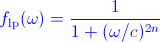

A few 1D low-pass filters with different c and n values are given in the figure below: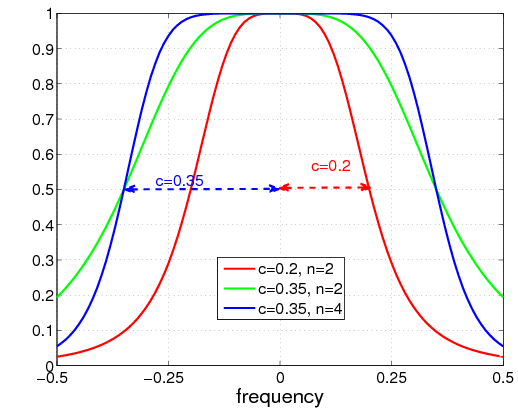

Note: This is a filter defined directly in the frequency domain. Do not confuse it with a Gaussian filter (for image smoothing in the spatial domain) where a broad profile means a larger standard deviation and more smoothing.

A high-pass filter f_hp can be defined as follows: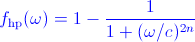

You can get low and high pass filter code from Professor Kovesi's website. You can use these functions to create 2D low-pass and high-pass filters. Download these functions and ensure that you understand how to call them. Note that the filters returned by these two functions are defined with the low frequency values at the beginning (i.e., corners) and end of the array. This conforms with the Fourier transform returned by Matlab's fft2 functions. A rule of thumb is therefore to stick to this convention and only use fftshift to swap the quadrants when you need to view the Fourier spectrum.

Sample image pairs

Some sample image pairs that you can use for your experiments are given below. Both images in each pair have the same dimension and have been aligned. Feel free to use your own image pairs. If you do so, include your images in your submission to cssubmit.

• woman (with neutral expression) and man (with angry expression)
• mouse and cat
• Obama and McCain

An example

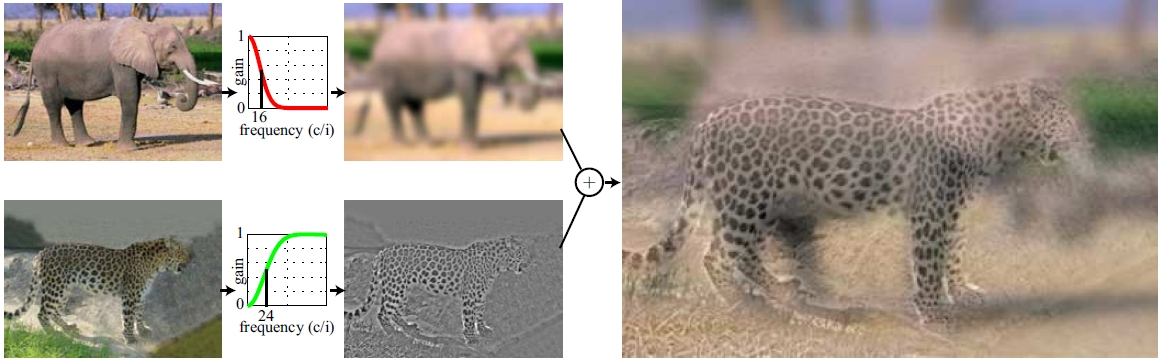
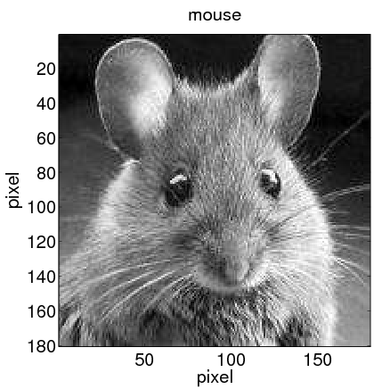
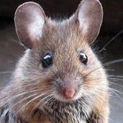
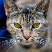
An example for generating a hybrid image is given below. The input image pair is the mouse.png and cat.png files. As these images are colour images, you should first convert them into greyscale, giving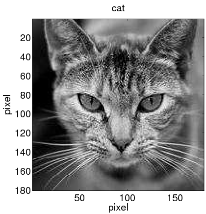

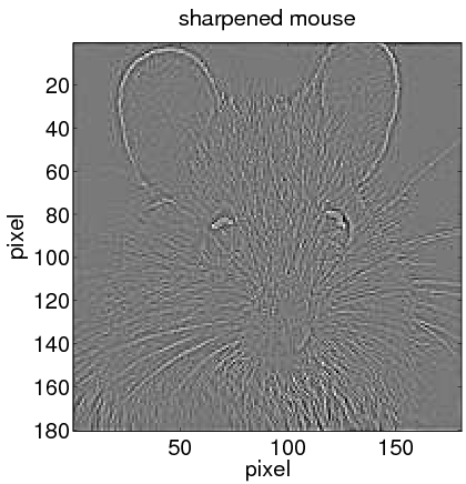
Design your low-pass filters and high-pass filters by selecting appropriate values for c and n. Ensure that the two filters do not cover a large common range of frequency values (see Figure 5(a) and (b) of reference [1] above and the related discussion there).

After applying your filters to the two images, it is a good practice to inspect the output smoothed and sharpened images before composing the hybrid image. For instance, your smoothed and sharpened images might look like this: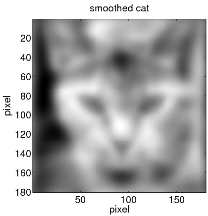

When the Fourier transforms of these two images are added and then inverse FFT back to the spatial domain, what you get is the desired hybrid image, which might look like: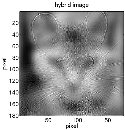

Hint:

• For the above example, try a small value n (e.g., 1, 2, or 3) for both filters. To ensure that the cat image is blurred enough to be seen only from afar, you need a very small cut-off c value, e.g., less than 0.1. For the high-pass filter, try a cut-off c value between 0.1 and 0.3.
• You can use Matlab's improfile to display the profile across the centre of each filter. For instance, if nrows and ncols are the numbers of rows and columns of the low-pass filter G, then improfile(G, [1 ncols], [round(nrows/2), round(nrows/2)]) would show the profile along the middle row of G. When no arguments is given to the improfile function, Matlab expects you to use the mouse to specify the start and end points of the cross section for the profile.
• An alternative to viewing the resultant hybrid image from a long distance away, you can halve the size of the image using subsample. The Matlab imresize function is handy for this. A reduced resolution image has the same effect as if the original image is viewed from afar.

You can try constructing colour (rather than greyscale) hybrid images if you have the time. However, greyscale images are sufficient for the exercises here.

Your tasks...

1. Write a Matlab script and save it to a file named test1.m. Demonstrate in the script file how you generate a hybrid image using two input images. Inspect the hybrid image at different distances. Adjust the values c and n of your low-pass and high-pass filters until the hybrid image reveals either input image when viewed at different distances.

   Your Matlab script should read in two input images, call the lowpassfilter and highpassfilter functions and construct the resultant image. Your code should display the resultant image (Hint: use imagesc and axis equal). When we mark your lab exercises, we will run your Matlab script and inspect the display. Apart from the resultant hybrid image, display intermediate images as well such as those shown in the example above to demonstrate your understanding of the hybrid image construction process.

2. Repeat the same process above for another pair of input images. Save the Matlab script to test2.m.

Submission Requirements

• your test1.m script file.
• your test2.m script file.
• your own image pairs (other than the sample ones supplied) that you use in test1.m and test2.m.

Apart from the lowpassfilter.m and highpassfilter.m files that you download from Assoc. Prof. Kovesi's website, other functions from his website that you use for this lab sheet must be included in your submission. We will test run your test1.m and test2.m files in the marking process. It is therefore important that your submission is complete.

Your Matlab code should be commented (but not over-commented) and indented for readability (Hint: Use the Matlab Editor to help you indent your code).