The Network Layer The Data Link Layer had the responsibility of reliably transmitting frames across along a single wire (or wireless, ...) link. The Network Layer's responsibility is to get packets from an actual source machine to a destination machine. There may be many hops along the way. The Network Layer is thus the lowest OSI Layer that has to deal with end-to-end transmission. The Network Layer must be aware of the immediate topology of its subnet (its neighbours) to make a routing choice that 'makes progress', avoids introducing congestion on links, and avoids already congested links. If the source and destination machine are on different networks (either physically or politically), we must support internetworking.   Network Layer Design Objectives The design objectives of an effective Network Layer are : to be independent of processor/communication technology, to be independent of the number, type and topology of the subnets, and to provide a uniform addressing scheme for all hosts in the network.

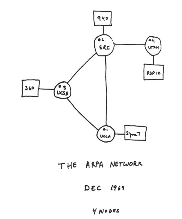
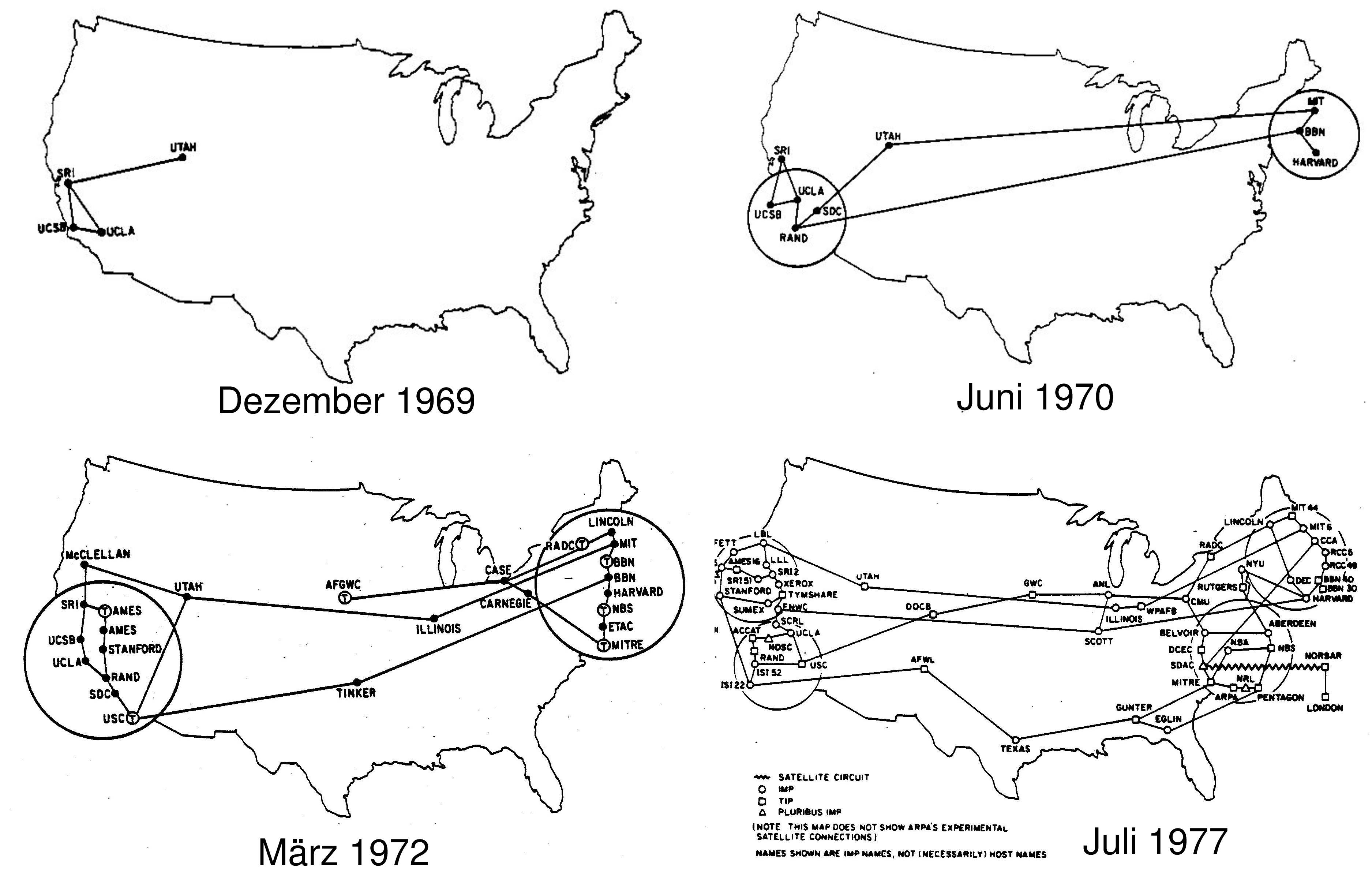
The Relationship Between Hosts and the Subnet

To place it in perspective, the Network Layer software runs in dedicated devices termed routers - early editions of Tanenbaum introduced the term IMPs (Intermediate Message Processors), and the Transport Layer (coming soon) runs in the hosts.

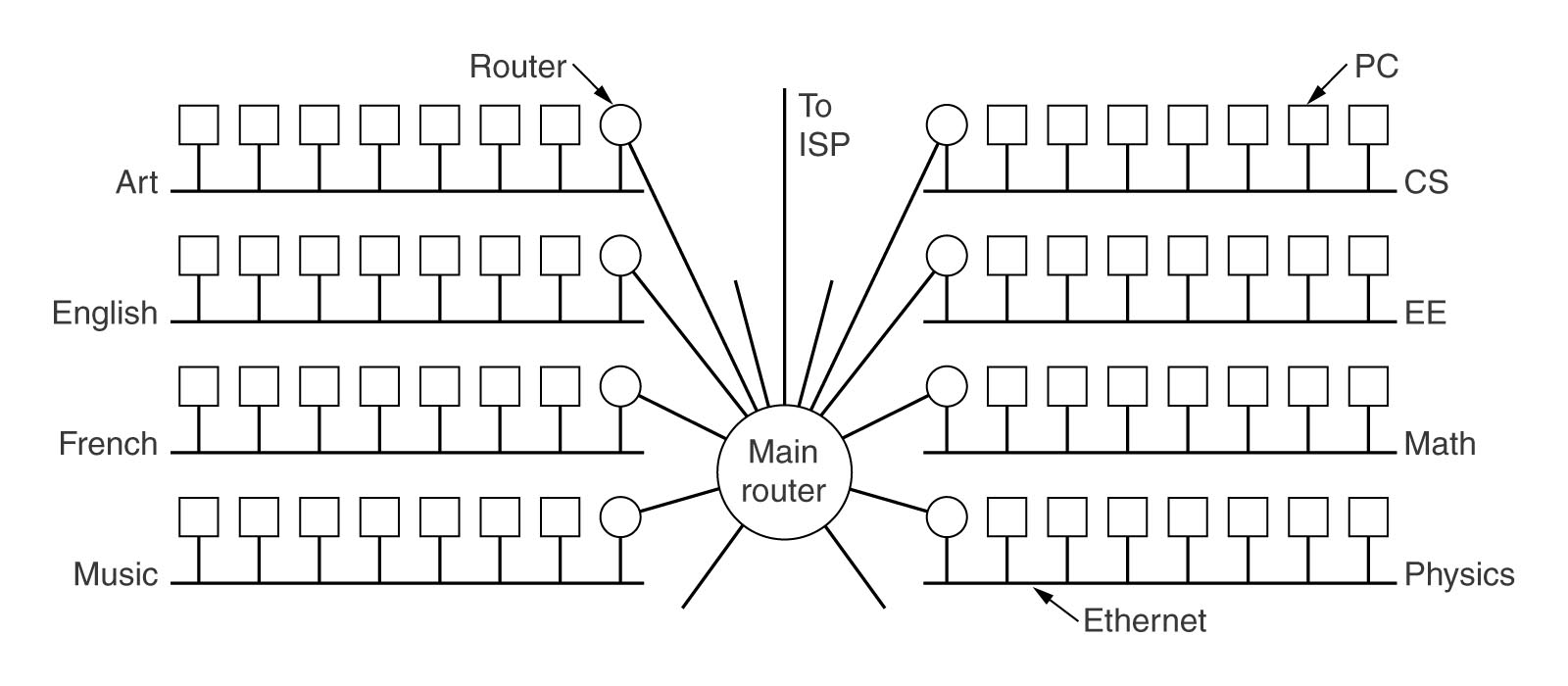Implications for Data Link Layer software

Except in the trivial 2-node case, some nodes will now have more than one physical link to manage.

When the Network Layer presents a packet (data or a control message) to the Data Link Layer, it must now indicate which physical link is involved.

Each link must have its own Data Link protocol - its own buffers for the sender's and receiver's windows and state variables such as ackexpected, nextframetosend, etc.

Responsibilities of the Network Layer The Network Layer includes nearly all of the functions we consider important in multi-node networks. Each node can be responsible for everything from handling its own links to managing (either guessing or knowing) the network topology. In essence, the requirements are of three types:

Source and destination functions:

end-to-end protocols, the network layer software interface, fragmentation and reassembly of messages, management of network layer sequence numbers, and creation, manipulation and deletion of headers.

Store and forward functions:

choice of the best route for packets, local flow control, and local error control.

Network-wide management functions:

network flow control, topological awareness and modification, and network performance measurement and monitoring.

An example NL responsibility - packet fragmentation and reassembly Messages may be divided into smaller data units, termed packets, before transmission. These packets may traverse the network independently until they reach the destination node. This requires fragmenting or segmenting the messages into packets at the source node and then reassembling the packets into messages at the destination. Furthermore, each packet's header must indicate that it is part of some bigger message. An important consideration for fragmentation is determining the 'optimal' packet size. Compared to variable-sized packets, fixed size packets offer a number of advantages: Throughout the network, each node's buffer size may be fixed. It is simpler to prevent congestion at a destination node, since the destination may accurately estimate the number of buffers to pre-allocate. Fixed-sized packets result in simpler memory allocation schemes - typically 'once-only' allocation can be used instead of constantly using 'random-sized' fully dynamic allocation. The primary disadvantage with fixed-sized packets is under-utilization of memory when the message size slightly exceeds an integral multiple of the packet size (for example, consider the very short last packet in the figure).

Network Layer Header Management

The Network Layer data unit, the packet, carries a Network Layer header which must serve many purposes.

The NL header is created in the source node, examined (and possibly modified) in intermediate nodes, and removed (stripped off) in the destination node.

The Network Layer headers typically contain (note that not all NL protocols will require or implement all of these fields or responsibilities):

• The source and destination node addresses,
• Packet size, if packets may be of more than one size,
• Message number, and possibly packet number within that message,
• Several control bits indicating if the packet is a 'user-data' packet or a control packet, whether or not fragmented, fixed or variable length,
• Flow control information, such as permission to send additional messages, or flags to change the rate of flow, and
• The packet priority.

Finally, the data portion (the payload) of the packet includes the 'user-data', control commands or network-wide statistics.

The Path of Frames and Packets

Whereas the Data Link Layer must acknowledge each frame once it successfully traverses a link, the Network Layer acknowledges each packet as it arrives at its destination.

Note the significant 'explosion' in the number of frames required to deliver each packet.

The Two Contending Network Layer Schemes

One community (the telecommunications companies) believe that all data should be transmitted reliably by the Network Layer.

Their proposal is for a connection-based service, termed a virtual circuit, in which : Before sending data, the Transport Layer should establish a 'semi-permanent' connection between the source and destination. The two Transport Layers then agree (argue) about the type and quality of service (QoS) that is required and will be available. Communication then occurs between the two parties in a duplex fashion along the acquired connection. The connection is then closed by both parties. Each routing device maintains tables of pairs of source and virtual circuit numbers and destination and virtual circuit numbers. The analogy here is with a telephone conversation. The connection-based service is often called a session-based service. See also: GettyImages: telephone switchboard operator

The Two Contending Network Layer Schemes, continued

They state that with this connectionless, datagram scheme, that the hosts must perform any required error processing. Thus error processing is 'relinquished' to the Transport Layer, above. that each host operates in a connectionless fashion in which each 'lump' of information is moved between source and destination without a permanent connection between them. that each packet moves independently of all previous packets between the same source and destination machines - with each packet possibly taking a different route. The result is that the only services provided by the Network Layer to the Transport Layer are to perform the operations of send packet and receive packet and no negotiation is possible.   The analogy here is with the postal service. Note that each packet must thus carry its full destination and source address.

Network Layer Routing Algorithms

The routing algorithms are the part of the Network layer software that decides on which outgoing line an incoming packet should go.

• For virtual circuits the route is chosen once for each session.
• For datagrams the route is chosen once for each packet.

Desirable properties for the routing algorithms are similar to those for the whole Network layer :

In particular, robustness often distinguishes between the two main classes of routing algorithms - adaptive and non-adaptive.

Robustness is significant for two reasons :

1. Once a large network is off and running it is difficult to change the routing algorithm software, and
2. Network topologies often change - hosts, IMPs and lines frequently fail.

The better a routing algorithm can cope with changes in topology, the more robust it is.

The Two Classes of Routing Algorithm

Non-adaptive Algorithms

are characterized by the fact that the choices of routes between each two hosts are computed in advance and loaded into each host in the whole network before the network is 'brought-up'.

Non-adaptive choices are often termed static routing.

Adaptive Algorithms

are characterized by their attempts to adjust their route choices based on their current knowledge of the network topology. There are three type of adaptive algorithms :

1. global algorithms use information periodically collected from the whole network (central routing),
2. local algorithms use only the information that each router knows about itself, such as queue lengths and waiting times, and
3. combined algorithms use some of both global and local information (distributed routing).

Adaptive choices are often termed dynamic routing.

Question: How do we know when a host, router or line has failed?

• Either the host (etc) tells us that it is about to shutdown, or
• We receive too many consecutive Network Layer timeouts for a destination host or router, or too many Data Link Layer timeouts for a link.

A naive non-adaptive routing algorithm - Flooding

Initially, every 'incoming' packet is retransmitted on every link:

void down_to_networklayer(/* event, timer, data */)
{
    READ_APPLICATION(/* get destn, msg and length */);

    // ... fill in packet header info

    for(int link=1 ; link<=NLINKS ; ++link) {
	DOWN_TO_DATALINK(link, packet, len);
    }
}


void up_to_networklayer(/* packet, length */)
{
    if(packet_is_for_this_node) {
	if(packet_is_data) {
	    WRITE_APPLICATION(/* the msg in the packet */);

	    // ... prepare acknowledgement

	    for(int link=1 ; link<=NLINKS ; ++link) {
		DOWN_TO_DATALINK(link, ... /* send ACK */);
            }
	}
	else {
	    ;  // ACK received => prepare to send more data
        }
    }
    else {     // send packet out again
	for(int link=1 ; link<=NLINKS ; ++link) {
	    DOWN_TO_DATALINK(link, packet, len);
        }
    }
}

Advantage : flooding gives the shortest packet delay (the algorithm chooses the shortest path because it chooses all paths!) and is robust to machine failures.

Improved Flooding Algorithms

Disadvantage : flooding really does flood the network with packets! When do they stop?

Partial Solutions :

• Do not retransmit packets on the link on which they arrived - they have already travelled from that direction.
• Each packet can include a hop count and after any hop count exceeds the diameter of the network the packet can be discarded.
• Acknowledgements need only be transmitted on the link on which the data packet arrived.
• As data packets arrive, each router can remember the link of minimum hop count on which it arrived - all subsequent packets for that destination go on that link.
• routers can keep a list of sequence numbers seen and if any packets are re-seen by any router they are discarded.

Examples: Three implementations of flooding are provided in .../resources/flooding.zip.
Please examine these as examples of Network Layer and Data Link Layer separation.

Adaptive Routing - Distance Vector Routing

Distance vector routing algorithms maintain a table in each router of the best known distance to each destination, and the preferred link to that destination.

Distance vector routing is known by several names, all descending from graph algorithms (Bellman-Ford 1957, and Ford-Fulkerson 1962). Distance vector routing was used in the wider ARPANET until 1979, and was known in the early Internet as RIP (Routing Information Protocol).

Consider the following:

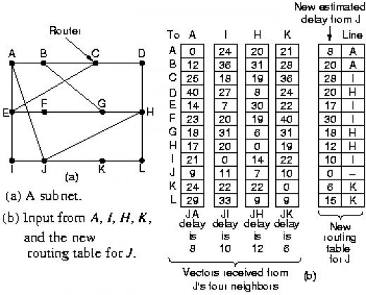Router J has recently received update tables from its neighbours (A,I,H,K) and needs to update its table. Note that J does not use its previous table in the calculations.

The Count-To-Infinity Problem

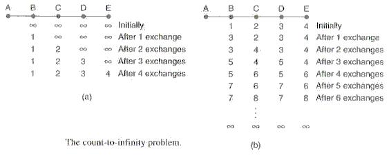When router A returns, each other router eventually hears of its return, one router at a time - good news travels fast.

However, consider the dual problem in (b). Router A is initially up. All other routers know the distance to A. Now, router A crashes - router B first senses that A is now an infinite distance away. However, B is excited to learn that router C is a distance of 2 to A, and so B chooses to now send traffic to A via C (a distance of 3).

At the next exchange, C notices that its 2 neighbours each have a path to A of length 3. C now records its path to A, via B, with a distance of 4. At the next exchange, B has direct path to A (of infinite distance), or one via C with a distance of 4. B now records its path to A is via C with a distance of 5.....

Adaptive Routing - Link State Routing

Initially, all ARPANET links were the same speed (56Kbps), and so the routing metric was just hops. As diversity increased (some links became 230Kbps or 1.544Mbps) other metrics were required. In addition, the growing size of the network exposed the slow convergence of distance vector routing. A simple example:

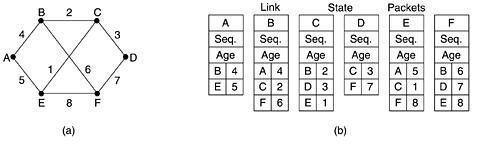Routers using link state routing periodically undertake 5 (easy to understand) steps:

1. Discover their neighbours' network addresses (send request packets, receive reply packets).
2. Measure the delay or cost to each of its neighbours (immediate delay, or queued delay?).
3. Construct link-state packets containing all just learnt.
4. Broadcast this packet to all neighbours (use a flooding variant to ensure quick propagation).
5. Compute the shortest path to each other router (perhaps using Dijkstra's shortest path algorithm).

Congestion and Flow-Control in the Network Layer

An additional problem to be addressed by the Network Layer occurs if too many packets are 'dumped' into some part of the subnet - network performance will degrade sharply.

Worse still, when performance degrades, timeouts and re-transmission of packets will increase.

Also, if all available buffer space in each router is exhausted, then incoming packets will be discarded (what??!!), causing further re-transmissions.

Congestion is both a problem that a node's Network Layer must avoid (not introduce), and must address (if other nodes' Network Layers cause it).

• Congestion control is concerned with ensuring that the subnet can carry the offered traffic - a global issue concerning all hosts and routers working together.

• Flow control is concerned with end-to-end control (possibly multiple hops apart).

The sender must not swamp the receiver, and typically involves direct feedback from the receiver to the sender to 'slow down'.

Congestion and Flow-Control, continued

Both congestion and flow-control have the same aim - to reduce the offered traffic entering the network when the load is already high.

Congestion will be detected through a number of local and global metrics -

• percentage of packets discarded for lack of buffer space,
• average router queue lengths,
• number of packets timing out requiring retransmission, and
• average (or standard deviation of) packet delay.

Open loop control attempts to prevent congestion in the first place (good design), rather than correcting it. Virtual circuit systems will perform open loop control by preallocating buffer space for each virtual circuit (VC).

• New VCs will not be created via an intermediate router is low on memory.
• A new VC may have to be created via another path.

Closed loop control maintains a feedback loop of three stages -

• monitoring of local subnet to detect where congestion occurs,
• passing information to where corrective action may be taken, and
• adjustment of local operation to correct problem.

End-to-end Flow Control

It is reasonable to expect conditions, or the quality of service, in the Network Layer to change frequently.

For this reason, the sender typically requests the allocation of buffer space and 'time' in the intermediate nodes and the receiver.

Packets are then sent in groups while the known conditions prevail.

Load Shedding

The term load shedding is borrowed from electrical power supplies - if not all demand can be met, some section is deliberately disadvantaged.

The approach is to discard packets when they cannot all be managed. If there is inadequate router memory (on queues and/or in buffers) then discard some incoming packets.

Load shedding must be performed under many constraints:

• Must balance 'reasonable delay' and 'user freedom'.
• Maintain fair access to the network for all users.
• Respect rights (privileges) of priority users.

A number of reasonable strategies exist for discarding packets:

• consider the priority of each packet (don't drop high priority packets). We also need a strategy to encourage senders to send low-priority packets.
• don't discard ACKs, throw out DATA instead.
• make packets carry a hop counter, don't discard a DATA packet if it has travelled a long way. Instead discard one that has only travelled a short distance.
• examine the type of traffic being carried (perhaps by its priority). File transfers must eventually see all frames - all discarded frames will be retransmitted. Discard frames with high sequence numbers, not low numbers. Multimedia data will likely not retransmit old frames, only new frames are of interest.

Traffic Shaping - Leaky Bucket Algorithm

Consider a leaking bucket with a small hole at the bottom. Water can only leak from the bucket at a fixed rate. Water that cannot fit in the bucket will overflow the bucket and be discarded.

Turner's (1996) leaky bucket algorithm enables a fixed amount of data to leave a host (enter a subnet) per unit time. It provides a single server queueing model with a constant service time.

If packets are of fixed sizes (such as 53-byte Asynchronous Transfer Mode cells), one packet may be transmitted per unit time. If packets are of variable size, a fixed number of bytes (perhaps multiple packets) may be admitted.

The leaky bucket algorithm enables an application to generate traffic which is admitted to the network at a steady rate, thus not saturating the network.

Traffic Shaping - Token Bucket Algorithm

The leaky bucket algorithm enforces a strict maximum traffic generation. It is often better to permit short bursts, but thereafter to constrain the traffic to some maximum.

The token bucket algorithm provides a bucket of permit tokens - before any packet may be transmitted, a token must be consumed. Tokens 'drip' into the bucket at a fixed rate; if the bucket overflows with tokens they are simply discarded (the host does not have enough traffic to transmit).

Packets are placed in an 'infinite' queue. Packets may enter the subnet whenever a token is available, else they must wait.

The token bucket algorithm enables an application to generate and transmit 'bursty' traffic (high volume, for a short period). It avoids saturating the network by only permitting a burst of traffic to continue for a limited time (until the tokens run out).